Google Sheets for Humanities Data: Conditional Formatting

Using Google Sheets to Organize and Manage Your Humanities Data

Workshop Series Topics

• Setting up your table
• Tool 1: Code tables
• Tool 2: Data Validation
• Tool 3: Conditional Formatting
• Tool 4: VLookup (coming soon!)
• Tool 5: Column Statistics & Filters (coming soon!)
• Tool 6: Pivot Tables (coming soon!)

If you’d like to download the full workshop presentation slides, you can find them here.

---

Welcome to Part 4 of my Google Sheets for Humanities Data workshop! If you’ve been following along with the series, you’ll already have learned how to create a spreadsheet from scratch, make a code (or reference) table, and enable data validation.

In this part of the workshop, the tool in focus is conditional formatting. Keep reading to learn more about how to jazz up the visual elements of your spreadsheets.

And remember, I’ve created a (fictional) sample dataset containing artworks and their locations across NYU residential halls in case you’d like to practice these skills but are worried about messing up your own data. Feel free to make a copy of this dataset!

About Conditional Formatting

Spreadsheets can contain enormous amounts of data. As a human working with numbers and text and functions, reading your spreadsheet can rapidly become quite overwhelming. While you can summarize this data in detail by using functions and creating pivot tables, there is a tool—conditional formatting—that enables you to gain insight about your sheet at a glance.

Conditional formatting lets you to specify conditions, or rules, to format particular elements in your spreadsheet. This feature works by using if/then statements to change the color or style of your cells and the text in them. Your sheet’s conditions, once applied, can be read as “if cell F3 contains exactly “Manhattan,” then color the text blue” or “if cells F2-F30 are empty, then color their backgrounds red.”

When working with large datasets, these minor edits will allow you to visually organize your sheets, making it easier for you to explore your data in seconds.

Potential uses of this tool include:

• Coloring text in every cell starting with letter “B” blue;
• Coloring cells’ backgrounds green if they contain values greater than or equal to 100;
• Italicizing text in cells containing (but not stating exactly) “Incomplete;”
• Applying a gradient in a column to signify values in a range between 50 and 50,000.

Tool 3: Conditional Formatting

Let’s get started!

With conditional formatting, you have the possibility of creating color-coded columns (as pictured above), highlighting certain pieces of text, and applying custom formulas and gradients to signify a range of data.

I’ve found this tool to be especially useful in my data workflows because, as a design-oriented individual, the visual elements in my spreadsheets help me get a better sense of what I’m working with. Just a quick glance at my colorful, but not overly bedecked, sheet allows me to see density, frequency, and patterns present in my data.

In this example above, taken from the sample (and fictional) dataset of artworks on view around NYU dorm halls, I’ve applied conditional formatting to color cells according to the city where the artwork venue is located.

Keep reading below to learn about the 3 components of this tool and how to apply it to your spreadsheet.

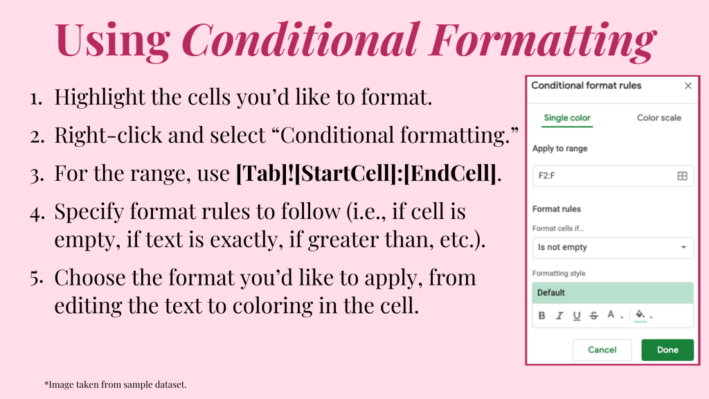
Once you’ve highlighted your desired cells and opened the conditional formatting settings, there are 3 elements to look out for:

• Range: The range refers to the cells where you’ll be applying your conditions. You can either type it in manually or click on the 4-cell grid symbol to select the range from your sheets.
  • Range format: [tab name]![start cell]:[end cell] –> Data!F2:F800 or Main!F2:F
    • These are read as “in tab Data, from cell F2 to F800” and “in tab Main, from cell F2 to every other cell in F.” If you’ll be working with an uncertain, but large, amount of data, simply typing the column name (F) allows you to encompass every cell that follows. I recommend starting in row 2 (F2) in order to exclude the column header/title from being formatted.
    • The exclamation mark signifies the end of the tab name and the colon signifies the range. If your document only includes one tab, you can omit the tab name and jump right to the cells (F2:F800).

• Format Rules: This is where you determine the conditions that will initiate particular formatting edits—the if clause. These rules will dictate what gets formatted in your sheets.
  • You can choose from a variety of rules according to what makes the most sense for your data.
    • Text-based rules: if text is exactly, if cell contains, if cell is empty, etc.
    • Numeric value-based rules: if date is before, if value is greater than, etc.
    • Custom formula: tailor your own function suit your organizational needs.

• Formatting Style: Once you’ve specified a range and rule, you must choose the formatting edit that will take place if your rules are met—the then clause.
  • Single color: if you prefer to designate individual colors for different conditions, choose Single color at the top of the settings box. You can edit your cells by formatting the text or the cell itself in various ways.
  • Color scale: if you’d like to apply a gradient or color scale to your data (as your formatting style), you can do so by selecting Color scale at the top of the settings box. From there, indicate which colors your gradient will include, your data’s minimum/maximum values, and what range will correspond to what color in the gradient.

To edit or delete any formats you’ve applied using this tool, highlight the range again and select “Conditional formatting.” You can edit rules by selecting each one and editing in the settings or delete rules by clicking on the little trash can symbol beside each one.

Your turn!

Give this tool a try, whether in the practice spreadsheet or your own sheets.

Try formatting the cells in column E to assign each hall name a different color of your choice. Once you’ve done that, the column should look quite colorful.

You can also try coloring cells with digit values (Artist BY, column D) using a scale to get a visual idea of which artists were born earlier and which were born later.

For a more detailed explanation of conditional formatting and its multiple functionalities, I recommend checking out this tutorial on Zapier.

---

Woohoo! You’ve just completed part 4 out of 7 of my Google Sheets workshop! Hopefully these tutorials and exercises have helped you to build your confidence in working with quantitative data in a software like Google Sheets.

Look out for my next tutorial: using the VLookup function to auto-populate cells. Though employing formulas in spreadsheet softwares can be intimidating, I’m going to help you get the basics down so that you can limit the amount of time and effort you spend filling your spreadsheet.

And, of course, feel free to share your thoughts and questions in the comments below (or via email!) 🙂